Neural Networks on House Prices
12 Aug 2017In the previous article, we used linear regression to predict the price of houses. Then, we saw that this model does not find any non-linear correlations. The most fascinating thing about neural networks is that they automatically model any non-linearities present in the phenomenon. In this article, we will use neural networks to overcome that shortcoming.
Note that this is a follow-up post. We already downloaded, and cleaned the Ames housing dataset in the previous article. If you haven’t done that already, you should probably go ahead and finish that first. In addition to that, we also split the dataset into 3 parts (training, validation, and testing). I will jump into the code assuming that’s already done. Or if you prefer, you can follow along by running the Jupyter Notebook.
All of the code used here is available in the form of a Jupyter Notebook which you can run on your machine.
What is a Neural Network?
As one might think, neural networks are systems that are modelled after the human nervous system. The human body has neurons that connected together is a very complex network, with each neuron branching out to many other neurons and getting input signals from multiple neurons. Similarly, in AI, neural networks can be thought of as inputs going to different temporary outputs, and those going to other temporary outputs, and so on until we lead the final temporary outputs to the final output. Each of these temporary outputs are called hidden layers because they don’t really expose themselves anywhere else.
The image (taken from Wikipedia) below will help you understand the flow of inputs to outputs.
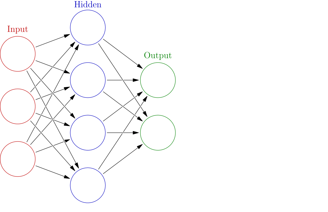
Notice that we are leading our features to multiple values. Think of each of these values as a separate linear problem (like the one we solved earlier). These new vector of values inside the hidden layer will now serve as new features for our problem. In this manner, we can construct many such hidden layers with different number of features. Finally, when we are happy, we can direct these features to the actual output. Generally speaking, more hidden layers equals better performance. But you must watch out for overfitting.
Notice that we described each of these connections as linear problems. That means they must have weights and biases. We find these parameters using a process called backpropagation. It’s called backpropagation because we use the final output and proceed in the direction towards the input (back) to reconstruct the weights and biases. The mathematics is a bit more complex than the one for linear regression and is beyond the scope of this article. Finally, we use an optimizer, just like Gradient Descent (in this tutorial we will be using Gradient Descent), to help converge the cost function.
An important aspect of neural networks is feeding the hidden layers into the next layer. It so happens that sometimes the gradient (when performing backpropagation) can vanish or explode. To prevent that we have activation functions. The most commonly used activation function is the Rectified Linear Unit function, abreviated as ReLU and is defined as follows:
f(x)=max(0,x)
It basically sets all negative values for the input to 0. This function also significantly speeds up our computation process.
Remember that a simple linear regression has two big drawbacks:
- The number of parameters are small and fixed
- They only model linear correlations
This is why neural nets (NN) have an edge over linear regression:
- There is great flexibility over the number of parameters (and hence performance). You can control the number of hidden layers and the number of nodes in each hidden layer.
- Since there are multiple layers each being activated by an ReLU, neural networks automagically model any non-linear correlations. The better your NN (not necessarily having more hidden layers), the more non-linear correlations it captures.
The Design of Our Neural Net
The NN we are going to create is a rather modest one. It has only one hidden layer. So, you can consider it more of a proof-of-concept that NNs are better than linear regression.
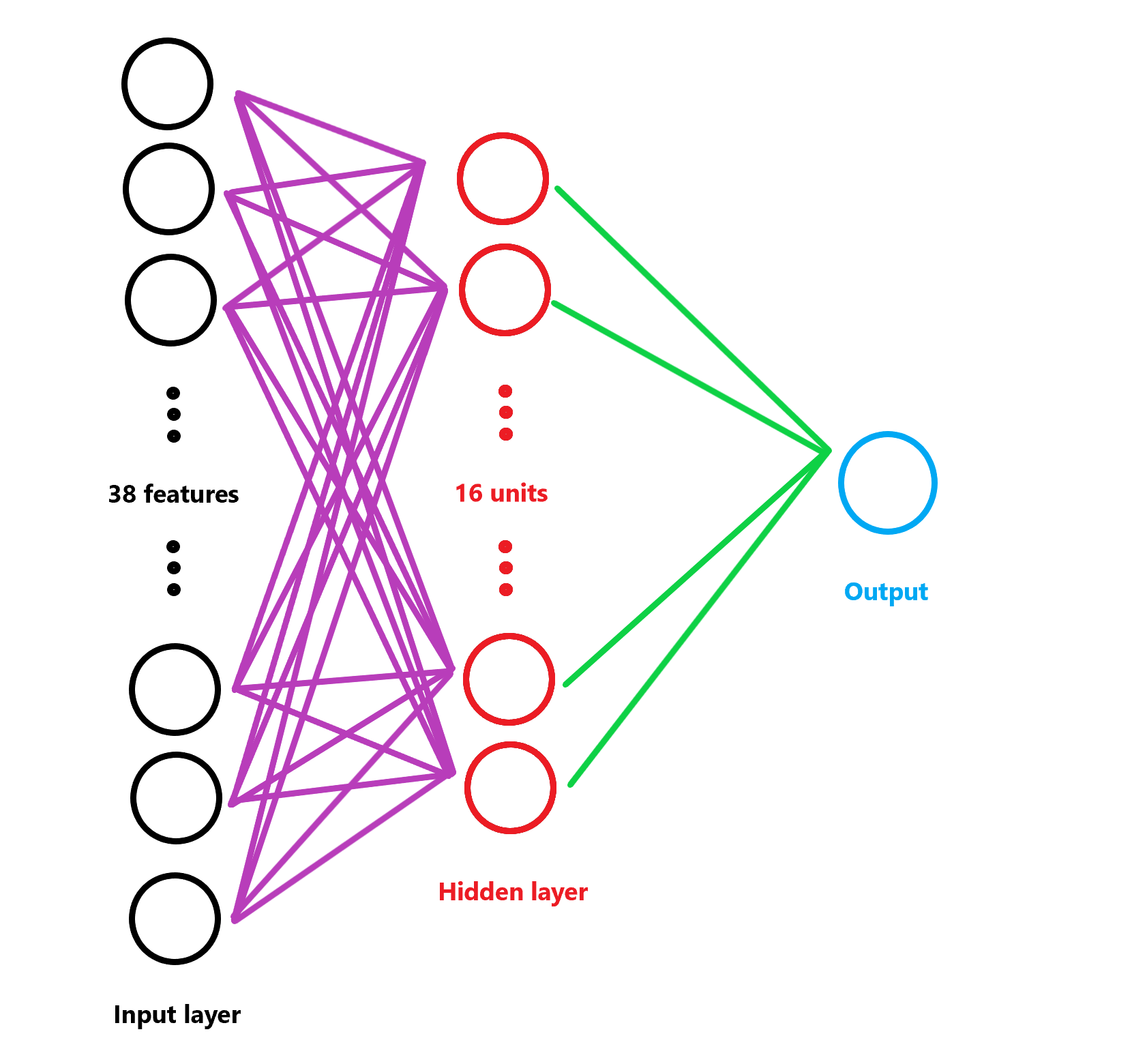
Our initial number of features is 38. So this is the size of our input layer. We will map this onto our hidden layer. Our hidden layer will have a size of 16. This hidden layer will undergo linear rectification with ReLUs. That will serve as features for our output.
The image below represents our NN
The neural network can be defined by these equations. Here, X is the input matrix, Wi and bi are weights and biases respectively. X2 represents the hidden layer, and y is the output.
x2=W1X+b1
Training the Neural Net
| import os | |
| import csv | |
| import numpy as np | |
| import pandas as pd | |
| import tensorflow as tf | |
| train_size = np.shape(x_train)[0] | |
| valid_size = np.shape(x_valid)[0] | |
| test_size = np.shape(x_test)[0] | |
| num_features = np.shape(x_train)[1] | |
| num_hidden = 16 # Number of activation units in the hidden layer | |
| # Neural network with one hidden layer | |
| graph = tf.Graph() | |
| with graph.as_default(): | |
| # Input | |
| tf_train_dataset = tf.constant(x_train, dtype=tf.float32) | |
| tf_train_labels = tf.constant(y_train, dtype=tf.float32) | |
| tf_valid_dataset = tf.constant(x_valid) | |
| tf_test_dataset = tf.constant(x_test) | |
| # Variables | |
| weights_1 = tf.Variable(tf.truncated_normal( | |
| [num_features, num_hidden]), dtype=tf.float32, name="layer1_weights") | |
| biases_1 = tf.Variable(tf.zeros([num_hidden]), dtype=tf.float32, name="layer1_biases") | |
| weights_2 = tf.Variable(tf.truncated_normal( | |
| [num_hidden, 1]), dtype = tf.float32, name="layer2_weights") | |
| biases_2 = tf.Variable(tf.zeros([1]), dtype=tf.float32, name="layer2_biases") | |
| steps = tf.Variable(0) | |
| # Model | |
| def model(x, train=False): | |
| hidden = tf.nn.relu(tf.matmul(x, weights_1) + biases_1) | |
| return tf.matmul(hidden, weights_2) + biases_2 | |
| # Loss Computation | |
| train_prediction = model(tf_train_dataset) | |
| loss = 0.5 * tf.reduce_mean(tf.squared_difference(tf_train_labels, train_prediction)) | |
| cost = tf.sqrt(loss) | |
| # Optimizer | |
| # Exponential decay of learning rate | |
| learning_rate = tf.train.exponential_decay(0.06, steps, 5000, 0.70, staircase=True) | |
| optimizer = tf.train.GradientDescentOptimizer(learning_rate).minimize(cost, global_step=steps) | |
| # Predictions | |
| valid_prediction = model(tf_valid_dataset) | |
| test_prediction = model(tf_test_dataset) | |
| saver = tf.train.Saver() | |
| # Running graph | |
| with tf.Session(graph=graph) as sess: | |
| tf.global_variables_initializer().run() | |
| print('Initialized') | |
| for step in range(num_steps): | |
| # Run the computations. We tell .run() that we want to run the optimizer, | |
| # and get the loss value and the training predictions returned as numpy | |
| # arrays. | |
| _, c, predictions = sess.run([optimizer, cost, train_prediction]) | |
| if (step % 5000 == 0): | |
| print('Cost at step %d: %.2f' % (step, c)) | |
| # Calling .eval() on valid_prediction is basically like calling run(), but | |
| # just to get that one numpy array. Note that it recomputes all its graph | |
| # dependencies. | |
| print('Validation loss: %.2f' % accuracy(valid_prediction.eval(), y_valid)) | |
| t_pred = test_prediction.eval() | |
| print('Test loss: %.2f' % accuracy(t_pred, y_test)) | |
| save_path = saver.save(sess, "./model/nn-model.ckpt") | |
| print('Model saved in %s' % (save_path)) | |
| # Reconstructing graph and predicting outputs | |
| with tf.Session(graph=graph) as sess: | |
| saver.restore(sess, "./model/nn-model.ckpt") | |
| print("Model restored.\nMaking predictions...") | |
| x = test_dataset.drop('Id', axis=1).as_matrix().astype(dtype=np.float32) | |
| hidden = tf.nn.relu(tf.matmul(x, weights_1) + biases_1) | |
| y = tf.cast((tf.matmul(hidden, weights_2) + biases_2), dtype=tf.uint16).eval() | |
| test_dataset['SalePrice'] = y | |
| output = test_dataset[['Id', 'SalePrice']] |
Continuing on after cleaning the data, we create some variables to store the size of the training data. Next, we define the number of activation units in out hidden layer as 16. Now, we are ready to construct our graph.
As in the previous case, we define the datasets as tf.constant because we don’t want to modify them in the graph.
Observe that we have two sets of weights and biases.
weights_1 and biases_1 map our input variables to the hidden layer. And the matrix sizes are defined in such a manner.
weights_2 and biases_2 map the hidden layer to the output.
Then we have steps. We’ll discuss this more when we move on to the optimzation.
Now, we define out model. This is simply a rendition of the mathematical equations we described earlier in TensorFlow style.
We do this for code reuse and readability.
Now, we compute the cost. The cost function we are using here is the same we used in the previous post.
So you can read that one to gain more insight.
Then we optimize and minimize the cost. This time, we are not using a fixed learning rate.
Instead, we exponentially decay the learning_rate i.e., as we run more iterations, the learning_rate slowly becomes smaller and smaller.
As we get closer to the minima, we start moving slower towards the minima to ensure that we do not miss it.
This is where the steps comes into play. This variable keeps track of the number of iterations.
And finally, the optimizer we use will be gradient descent.
Finally, we use our parameters and predict the output for the test and validation dataset.
Now, we are ready to train our model. We initiate a tf.Session with our graph and run the graph for 1000000 steps.
If you do not have access to tensorflow-gpu, I recommend you reduce the number of iterations for faster results.
After running, we save our weights and biases for later use.
You may want to read the previous post for a line by line code description.
Results
We first reconstruct our graph by initiating a tf.Session and restoring variables from the checkpoint file.
Then we predict the sale prices of the test data from these weights and biases.
Remember to predict the output using the same model you used to train.
Here is a graph comparing the actual values (blue) and predicted values (orange).
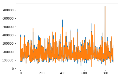
This model has a score of 2.23802. This is a slight improvement from linear regression.
And this should place a few hundred ranks above your previous rank on the leaderboards.
Scope for Improvement
As you can see, there is still room for improvement. In fact, we started out saying that NNs are, generally speaking, better than linear regression and our NN was only slightly better than the linear regression. Here are some things you can do to make the NN better:
- Better feature engineering - Here is a list of things you can do to have better features:
- Keep more features. We dropped lots of features. I bet there is some correlation between these features and the sale price.
- Creating bins instead of using actual features can prevent overfitting.
- Better cost function - The cost function we used does not take the large range of sale prices into consideration. Think about it this way - we penalized the model for predicting a $5000 house to be $0 (i.e., a difference of $5000) by the same amount if it predicted a $200,000 house to be $150,000 (i.e., a difference of $5000). We know that this is wrong. Instead, you can define a new function that computes the square difference of log.
- Prevent overfitting - You can use regularization to prevent this. In fact, in NN, there is more sophisticated method called Dropout. My guess is that this won’t work well because our training data is small. But you should definitely check it out.
- Go deeper - Try experimenting with multiple hidden layers and vary the number of activation units in each layer. This is really just a shot in the dark, but you never know what’s going to turn up!
Final Words
I think this is a really great hands-on experience to get your feet wet with machine learning and TensorFlow. If you have any questions, or see any factual inaccuracies, let me know in the discussion below or contact me. I plan on writing more tutorials, especially for the other two Getting Started Kaggle Competitions. If you think you’d want to read those, subscribe to the RSS feed and stay updated.