Regression on House Prices
31 Jul 2017Linear regression is perhaps the heart of machine learning. At least where it all started. And predicting the price of houses is the equivalent of the “Hello World” exercise in starting with linear regression. This article gives an overview of applying linear regression techniques (and neural networks) to predict house prices using the Ames housing dataset. This is a very simple (and perhaps naive) attempt at one of the beginner level Kaggle competition. Nevertheless, it is highly effective and demonstrates the power of linear regression.
All of the code used here is available in the form of a Jupyter Notebook which you can run on your machine.
Pre-requisites
This article assumes the reader to be fluent in Python to understand the code snippets. At least a strong background in other programming languages should be necessary. We will build our models using Tensorflow. So basic knowledge Tensorflow would be helpful, but is not a necessity. The tutorial also assumes the reader is familiar with how Kaggle competitions work.
The Raw Data
First off, we will need the data. The dataset we will be using is the Ames Housing dataset and can be downloaded from here.
Opening up the train.csv, you will notice nearly 52 features of 1460 houses.
What each of these features represent is described in data_description.txt.
The file test.csv differs from train.csv in that there are fewer houses and the prices for each of the houses is not present.
We will use the train.csv file to train and build our model.
Then, using that model, we will predict the prices for each of the houses in test.csv.
You might want to spend some time studying this data by graphing charts, etc. to gain a better understanding of the data. This will definitely be helpful, but we will not do that here.
Cleaning Data
The cleaning of data refers to many operations. Here we will be performing feature engineering (creating new features), filling in missing values, feature scaling, and feature encoding.
| import csv | |
| import random | |
| import numpy as np | |
| import pandas as pd | |
| def cleanup(df): | |
| ''' | |
| Cleans data | |
| 1. Creates new features: | |
| - total bathrooms = full + half bathrooms | |
| - total porch area = closed + open porch area | |
| 2. Drops unwanted features | |
| 3. Fills missing values with the mode | |
| 4. Performs feature scaling | |
| ''' | |
| # Features to drop | |
| to_drop = ['MiscFeature', 'MiscVal', 'GarageArea', 'GarageYrBlt', 'Street', 'Alley', | |
| 'LotShape', 'LandContour', 'LandSlope', 'RoofMatl', 'Exterior2nd', 'MasVnrType', | |
| 'MasVnrArea', 'BsmtCond', 'BsmtExposure', 'BsmtFinType1', 'BsmtFinType2', | |
| 'BsmtFinSF1', 'BsmtFinSF1', 'BsmtUnfSF', 'TotalBsmtSF', 'Heating', 'Electrical', | |
| 'LowQualFinSF', 'GrLivArea', 'BsmtFullBath', 'BsmtHalfBath', 'FullBath', | |
| 'HalfBath', 'KitchenQual', 'TotRmsAbvGrd', 'Functional', 'FireplaceQu', | |
| 'GarageType', 'GarageFinish', 'GarageQual', 'PavedDrive', 'WoodDeckSF', 'OpenPorchSF', | |
| 'EnclosedPorch', '3SsnPorch', 'ScreenPorch', 'PoolQC', 'MoSold'] | |
| df['Bathrooms'] = df['FullBath'] + df['HalfBath'] | |
| df['PorchSF'] = df['EnclosedPorch'] + df['OpenPorchSF'] | |
| df = df.drop(to_drop, axis=1) | |
| # Columns to ignore when normalizing features | |
| to_ignore = ['SalePrice', 'Id'] | |
| for column in df.columns: | |
| x = df[column].dropna().value_counts().index[0] | |
| df = df.fillna(x) | |
| if df[column].dtype != 'object' and column not in to_ignore: | |
| m = df[column].min() | |
| M = df[column].max() | |
| Range = M - m | |
| df[column] = (df[column] - m) / Range | |
| return df | |
| def encode_features(df_train, df_test): | |
| ''' | |
| Takes columns whose values are strings (objects) | |
| and categorizes them into discrete numbers. | |
| This makes it feasible to use regression | |
| ''' | |
| features = list(df_train.select_dtypes(include=['object']).columns) | |
| df_combined = pd.concat([df_train[features], df_test[features]]) | |
| for feature in features: | |
| unique_categories = list(df_combined[feature].unique()) | |
| map_dict = {} | |
| for idx, category in enumerate(unique_categories): | |
| map_dict[category] = idx + 1 | |
| df_train[feature] = df_train[feature].map(map_dict) | |
| df_test[feature] = df_test[feature].map(map_dict) | |
| return df_train, df_test |
52 features is a bit overwhelming. And if you have spent time studying what each of these features represent, you’d probably say that many of the features are redundant to some extent i.e., they play a very small role in the price of a house. So the first thing we will do is remove these features and make life simpler. The code snippet describes the features we want to get rid off. But, before we remove them forever, notice that the total porch area and total number of bathrooms is split into 2 columns. Again, to make life simpler, we will combine them into a single total porch area and a single total number of bathrooms. Now, we can go ahead and get rid off all these unwanted features.
The next thing we want to do is handle missing values. There are various ways to tackle this problem. An aggressive approach is to remove that entire training example. This can be bad if there are lots of missing values because you will lose too much data. But then, why would you train a model if you think you don’t have enough data? A simple and effective approach is to replace the missing value with mode (the most frequent value taken by that feature). A more sophisticated (and maybe better) technique is to study the other features and determine the missing value using probability and statistics. You might have guessed it - we are going to deal with missing values be replacing it with the mode.
The next thing we want to do is scale down the features. The motivation behind this is that some of our features have a large range of values. And this makes it difficult for our optimizer to converge. But, more on that later. We will use the following method for rescaling.
x′i=xi−min(X)max(X)−min(X)
Here, xi is the ith example of the feature X and, min(X) and max(X) refer to the minimum and maximum values the feature X takes respectively. An important thing to note is that you do not want to scale the output i.e., the Sale Price. This can lead to large errors in output and leave you clueless for a long time.
In machine learning, we almost always deal with numbers. But many of the features have letters for values where each letter (or sequence of letters) refer to a particular category. This is true for many datasets. And it also makes life difficult for us. And we do not like it when life becomes difficult. So, we will encode each of these features i.e., we will map a one-to-one correspondence from each of these categories to a number. The code snippet demonstrates how we achieve this.
The data we have now is almost ready for training.
Splitting Dataset
A standard practice is to split the data into 3 parts - training, validation and test datasets. We will use the training dataset alone to actually train the model. Then we will use the errors the model gives on the validation dataset to tune our hyperparamters. But now, the model we trained has “seen” the validation dataset. This means that if we were to report the error the model produced using either the training or validation datasets, our real error would be biased because this model has been exposed and modified to minimize the error on these datasets. This is where the test dataset comes into play. Its purpose is to serve as an unbiased judge and report the error on the model.
Usually, the dataset is divided as 60% training, 20% validation and 20% testing. And we will follow that fashion. We will also shuffle the dataset to make sure data is equally distributed across the 3 datasets.
So far we have been dealing with pandas dataframes. Alas! Tensorflow likes numpy arrays better.
So, we will have to fix that by converting the dataframes into matrices.
While doing so, we also need to separate the inputs, X, and outputs, y.
| def split(train_dataset): | |
| ''' | |
| Shuffle data and split into 3 datasets | |
| 1. Training - 60% | |
| 2. Validation - 20% | |
| 3. Testing - 20% | |
| ''' | |
| # Shuffle data | |
| train_dataset = train_dataset.sample(frac=1) | |
| train, valid, test = np.split(train_dataset, | |
| [int(.6 * len(train_dataset)), int(.8 * len(train_dataset))]) | |
| # Convert into numpy arrays | |
| x_train = train.drop(['SalePrice', 'Id'], axis=1).as_matrix().astype(np.float32) | |
| y_train = train['SalePrice'].as_matrix().astype(np.float32).reshape((np.shape(x_train)[0], 1)) | |
| x_test = test.drop(['SalePrice', 'Id'], axis=1).as_matrix().astype(np.float32) | |
| y_test = test['SalePrice'].as_matrix().astype(np.float32).reshape((np.shape(x_test)[0], 1)) | |
| x_valid = valid.drop(['SalePrice', 'Id'], axis=1).as_matrix().astype(np.float32) | |
| y_valid = valid['SalePrice'].as_matrix().astype(np.float32).reshape((np.shape(x_valid)[0], 1)) | |
| return x_train, y_train, x_test, y_test, x_valid, y_valid |
Linear Regression
The Algorithm
As I mentioned earlier, linear regression is perhaps the heart of machine learning. And the algorithm is the equivalent of the “Hello World” exercise. The algorithm is a very simple linear expression.
Y=WX+b
Here, Y is the output values for X, the input values. W is referred to as the weights and b is referred to as the biases. Note that Y and b are vectors and W and X are matrices. This is, in many ways, analogous to the line equation in 2 dimensions you might be familiar with.
y=mx+c
The only difference is that we are extending and generalizing this relation to n dimensions. Just like being able to find a line equation between two points i.e., calculation m and c, we are going to find the weights W and biases b.
In this way, we are going to map a linear relation between the sale prices and the features. It is important to stress on the fact that this is only a linear relationship. In reality, very few events are linearly correlated.
Naturally the question we have is figuring out the weights and biases. To do this we will first randomly initialize the weights, and initialize the biases to 0. Then we will calculate the right hand side of the equation and compare it with the left hand side. We will define the error between them as the Cost or, the more commonly used term in neural networks, loss.
loss=12n∑i=0((Y)−(WX+b))2
Then, this becomes an optimization problem where we are trying to find W and b to minimize the loss. There are various methods to optimize this. As usual we will stick with the simpler one - Gradient Descent Optimizer. Understanding this optimizer is perhaps beyond the scope of this article. But imagine optimizing a function in one variable using derivatives and generalizing that method to a function n variables. That is the core of gradient descent.
Now, let’s jump into the code.
The Implementation
| import tensorflow as tf | |
| import numpy as np | |
| def accuracy(prediction, labels): | |
| return 0.5 * np.sqrt(((prediction - labels) ** 2).mean(axis=None)) | |
| train_size = np.shape(x_train)[0] | |
| valid_size = np.shape(x_valid)[0] | |
| test_size = np.shape(x_test)[0] | |
| num_features = np.shape(x_train)[1] | |
| # Linear Regression Graph | |
| graph = tf.Graph() | |
| with graph.as_default(): | |
| # Input | |
| tf_train_dataset = tf.constant(x_train, dtype=tf.float32) | |
| tf_train_labels = tf.constant(y_train, dtype=tf.float32) | |
| tf_valid_dataset = tf.constant(x_valid) | |
| tf_test_dataset = tf.constant(x_test) | |
| # Variables | |
| weights = tf.Variable(tf.truncated_normal([num_features, 1]), dtype=tf.float32, name="weights") | |
| biases = tf.Variable(tf.zeros([1]), dtype=tf.float32, name="biases") | |
| # Loss Computation | |
| train_prediction = tf.matmul(tf_train_dataset, weights) + biases | |
| loss = 0.5 * tf.reduce_mean(tf.squared_difference(tf_train_labels, train_prediction)) | |
| cost = tf.sqrt(loss) | |
| # Optimizer | |
| # Gradient descent optimizer with learning rate = alpha | |
| alpha = tf.constant(0.01, dtype=tf.float64) | |
| optimizer = tf.train.GradientDescentOptimizer(alpha).minimize(loss) | |
| # Predictions | |
| valid_prediction = tf.matmul(tf_valid_dataset, weights) + biases | |
| test_prediction = tf.matmul(tf_test_dataset, weights) + biases | |
| saver = tf.train.Saver() | |
| # Running graph | |
| num_steps = 100001 | |
| with tf.Session(graph=graph) as sess: | |
| tf.global_variables_initializer().run() | |
| print('Initialized') | |
| for step in range(num_steps): | |
| # Run the computations. We tell .run() that we want to run the optimizer, | |
| # and get the loss value and the training predictions returned as numpy | |
| # arrays. | |
| _, c, predictions = sess.run([optimizer, cost, train_prediction]) | |
| if (step % 5000 == 0): | |
| print('Cost at step %d: %f' % (step, c)) | |
| # Calling .eval() on valid_prediction is basically like calling run(), but | |
| # just to get that one numpy array. Note that it recomputes all its graph | |
| # dependencies. | |
| print('Validation loss: %.2f' % accuracy(valid_prediction.eval(), y_valid)) | |
| t_pred = test_prediction.eval() | |
| print('Test loss: %.2f' % accuracy(t_pred, y_test)) | |
| save_path = saver.save(sess, "./model/linear-model.ckpt") | |
| print('Model saved in %s' % (save_path)) | |
| # Reconstructing model and predicting outputs | |
| with tf.Session(graph=graph) as sess: | |
| saver.restore(sess, "./model/linear-model.ckpt") | |
| print("Model restored.\nMaking predictions...") | |
| x = test_dataset.drop('Id', axis=1).as_matrix().astype(dtype=np.float32) | |
| y = tf.cast((tf.matmul(x, weights) + biases), dtype=tf.uint16).eval() | |
| test_dataset['SalePrice'] = y | |
| output = test_dataset[['Id', 'SalePrice']] |
In Tensorflow, we first define and implement the algorithm in a structure called graph.
The graph contains our input, output, weights, biases, and the optimizer.
We will also define the loss function here. Then, we run the graph in a session.
During each iteration, the optimizer will update the weights and biases based on the loss function.
In our graph, we first define the train dataset values and labels (output), the validation and testing datasets.
Note that we are defining them as tf.constant. This means that these “variables” will not and can not be modified when the graph is running.
Next, we initialize the weights and biases. We treat these as tf.Variable.
Pay attention to the dimensions of these matrices. You will run into compilation errors if you get them wrong.
This means that these “variables” have the capacity to be updated and modified during the course of our session.
Now, we predict the Y values using the weights and biases using the tf.matmul() function.
This is nothing but matrix multiplication. Then we add that to biases.
But if you go back to the definition, biases is a single number while tf.matmul(tf_train_dataset, weights) is a vector.
This might be confusing because you can only add a vector to another vector.
But Tensorflow is quite clever. It understands that we mean to add the same scalar biases to each element of the vector.
Think about this as converting the single number into a vector (or matrix) of same dimensions as the other vector,
and then adding those together. This is called broadcasting.
Then we calculate the loss as we defined previously. We can safely ignore cost for now.
It’s only purpose is to report the error we get.
When using the gradient descent optimizer, we need a parameter (one of the hyperparamters) called learning rate.
The term is self explanatory - it refers to how fast we want to minimize the loss.
If it’s too big, we will only keep increasing the loss. If it’s too small, and the algorithm will converge very slowly.
Here, we define alpha as the learning rate. After much experimentation, I’ve decided to use 0.01 as the learning rate.
It might be beneficial to vary this value and test for yourself.
Next, we define the optimizer. As mentioned earlier, we are using gradient descent with a learning rate alpha
and trying to minimize loss. This will update the tf.Variable elements involved in the calculation of loss.
After that, we are predicting the outputs on the validation and testing datasets using the new weights and biases.
Finally, notice the saver. What this does is it saves the weights, biases, and all other tf.Variable into a checkpoint file.
We can use these at a later stage to make our predictions.
That is how our graph is constructed. Now, we can run the graph in our session.
We start our session by initializing the global variables. This means initializing all tf.Variable.
Then we use the .run() function to run the session for 100000 steps.
Generally, the more number of steps, the better your results.
But 100000 can seem like a large number and will take a long time if you can’t make use of GPU.
If that is your case, you can either install tensorflow-gpu or just reduce num_steps to 10000.
After each run, we are storing the cost and train_predictions locally outside the graph.
And after every 5000 steps, we are calculating the cost of out model on the validation dataset.
At the end of the run, we save the session using the saver we created in the graph.
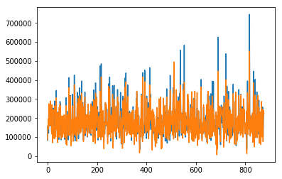
These are my results after 100000 iterations. The blue line is the actual value and the orange line is the predicted value.
It’s quite impressive that such a simple idea can yield really good results.
There is still lots of room for improvement though. I will touch upon some of those ideas at the end.
The Prediction
Finally, we are ready to predict the prices of houses whose features are described in test.csv.
First, we initialize a new session. Then we restore the variables from the saver.
And using these restored weights and biases, we predict the output on the new dataset.
You can save that into a .csv file and make a submission.
You should get a score of 2.5804. And you should be placed in the top 2000 ranks (as of 31 Jul 2017).
Improvements to Linear Regression
As I mentioned earlier (and as you might have guessed) there is certainly room for improving this naive model. Here are a few ideas to think about:
-
Regularization - This concept is very very important to make sure your model doesn’t overfit the training data. This might lead to larger errors on the training set. But, your model is bound to generalize better outside your training set. This means that your model is more likely to be applicable in the real world if you use regularization.
-
Creating bins - Remember how each of the numerical features (like area) are such varying numbers. To prevent overfitting, you can create bins for these features. For instance, all houses with area between 1000 and 1500 sq. ft would be assigned a value of 1 (say). I have seen this idea work really well for classification problems.
-
More features - I dropped a lot of features reasoning out that they wouldn’t cause the house price to be affected. In reality, I have no basis for that “fact”. Actually, there is a good chance they there is at least a correlation (if not a causation) between them. And any correlation, no matter how small, will help your model. So don’t drop them. Keep them around and test. You can even try your hand at engineering new features that you think might be helpful.
-
A new cost function - Did you notice the range of house prices? The cost function we used did not take this into consideration. Think about it this way - we penalized the model for predicting a $5000 house to be $0 (i.e., a difference of $5000) by the same amount if it predicted a $200,000 house to be $150,000 (i.e., a difference of $5000). We know that this is wrong. Instead, you can define a new function that computes the square difference of log. This will fix the problem of the large range of output values.
-
Non-linearities - Our assumption was that the output was linearly related to these features. This is rarely the case. One way to fix that is randomly try creating new features X′ from X where X′=Xn (n is another random number) and testing it out. This is clearly impossible and infeasible. One of the reasons why neural networks are amazing is that they automagically identify and map these non-linearities.
Next Steps…
This post is already longer than I intended it to be. And at the same time, I feel that making this shorter would make it less adequate. So, the next article will continue on our discussion of the Ames housing data. And in the next article, we will be using neural networks and see why it can be a better approach. Meanwhile, the code for the neural network is already out there. So you are welcome to continue using the Jupyter Notebook to try out neural networks.